Generating Smooth Connections in 3D Mesh Models of Brain Arteries
By Wojciech Malara
In the previous articles in this series my colleagues described some challenges we faced regarding processing of 3D mesh models of brain aneurysms. One of them was to automatically generate connections from the inlet and outlet branches of an aneurysm to some external points.
Whereas that article described the process of finding the starting points of that connection on the vessel model, in this article I am going to focus on the next step, i.e. generating the actual mesh and appending it to a model in a seamless manner.
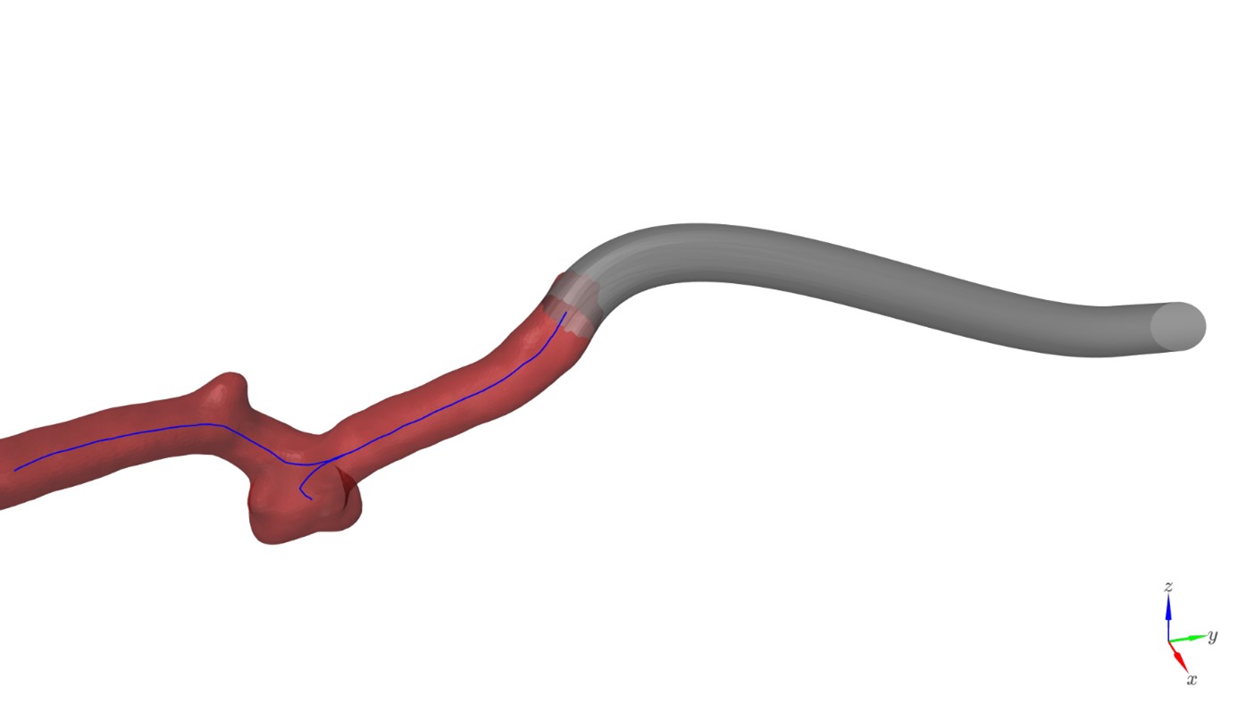
Figure 1. The original model of a vessel (red) with centerlines (blue) and the generated connection (gray)

Figure 2. The original model of a vessel cut and merged with the generated connection
Connection spline
The first step towards creating connections is generating paths along which connection “tubes” should be placed. In fact, these paths are centerlines of the connections. At this stage all vessels have centerlines generated and on each branch there is a certain point selected to be the start of a connection. In order to ensure that connections are seamless we decided to use cubic B-splines in which the starting part is tangent to a centerline at the selected point and the ending is tangent to a configured vector.
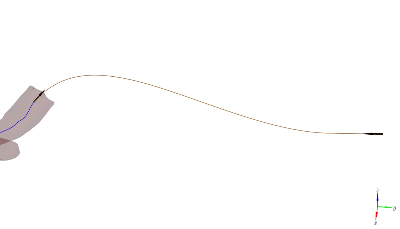
Figure 3. Generated connection spline with starting and ending vectors
There is one more crucial requirement for these connections. Not only should they be smooth in terms of the starting and ending vectors but the generated 3D mesh itself should be connected with the original anatomy seamlessly. This means it should start with the exact contour of a branch cross-section and transition smoothly into a target circular shape.
The solution to this requirement can be divided into following steps:
1. cut a vessel at a certain point,
2. get a contour of the section,
3. “sweep” the contour along the generated spline,
4. modify the swept contour to ensure that it transitions into a circle,
5. generate the actual mesh,
6. connect the generated 3D mesh with the cut vessel.
In the subsequent parts of this article I am going to describe each of these steps in detail, focusing in particular on the most interesting ones for us, i.e. “sweeping” a shape along a path and making it transition to a circle.
Cutting a vessel at a certain point
The task of cutting a vessel mesh at a certain point may seem trivial as we take a vector tangent to a centerline at this point and use it as a normal vector of a cutting plane. This approach isn’t ideal for branching vessels. The plane cut likely slices through other vessel parts. A disc might be better, but finding the right radius is tricky. Even then, nearby vessel sections could still be cut. Thankfully, in Graylight Imaging we have a common and ever-growing set of programming libraries with solutions to common problems. In this case, we used a tool which returns a polygon cross-section of a vessel at a certain point of its centerline. Then you can use this slice to cut the mesh by looking at how these meshes collide with each other.
Obtaining a section contour
Another important piece of data obtained from the aforementioned collisions analysis is boundary vertices and edges known almost right away by looking at colliding cells of the vessel mesh lying in the half-space indicated by a vector opposite the normal defining the cut. These boundaries form a “loop” which can be used as a starting shape for sweeping of the connection from the vessel to the target point and shape.
“Sweeping” a contour along path
How to sweep a contour along some path in 3D? Let’s start with the simplest idea: translating the contour into consecutive points on the curve. Straight lines work with this approach, but it fails elsewhere. Here’s why: The normal vector, defining contour orientation, must be tangent to the curve at every single point. This method breaks that rule for non-straight lines.
Straight lines are easy, but for curves, we need more than just location. In other words, we have to consider the orientation of the curve at each point. To achieve this, for each point (except the first with known orientation), calculate the tangent vector and the vector to the previous point. This captures orientation along the curve. Then, we calculate the angle between these two vectors and the cross product of these vectors in order to get a vector perpendicular to them. This way we have all the rotations between the consecutive points in axis-angle representation. Having all this information, we can use e.g. Rodrigues’ formula to rotate the contour’s vertices at each path point sequentially. This solution was almost perfect, but with one hitch. The issue? We started each point’s rotation from the previous one. For long, curvy paths, this caused errors to build up. As a result, the final point’s orientation sometimes wasn’t perfectly perpendicular to the tangent vector.
Simple matrix multiplication
As a result, we came up with a better idea which was also based on the tools we already had in our “toolbox”. The solution was to generate a moving frame (orthonormal basis) at each point on the curve. We used an idea similar to Frenet-Serret frame [1], but with more stable normal vectors. With all the basis vectors in hand, we built change-of-basis matrices for each point on the path. This allowed us to convert contour points to these bases directly using simple matrix multiplication.
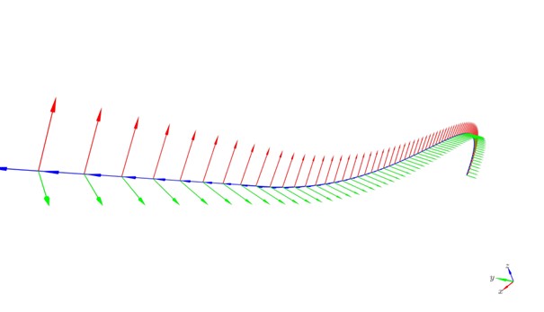
Figure 4. Bases along the connection spline points
Transforming a contour into another shape during “sweeping”
As mentioned before, not only did we have to create a connection starting from the contour of a vessel cross-section, but the contour should also transition into a different shape smoothly along a given path. In our case, the final shape was probably the simplest one – a circle, but the idea presented here can be utilized for almost any other 2D shape as well. The idea is simple: take each vertex of the starting contour and assign a position on a final shape to it in the same coordinate system, then use e.g. a linear interpolation to create intermediate positions for each vertex at each step (path point). To move these vertices to the appropriate positions in 3D space, we use the change-of-basis matrices described in the previous section. It is worth mentioning that in some cases it might be necessary to increase the resolution of the starting polygon by subdividing its segments.
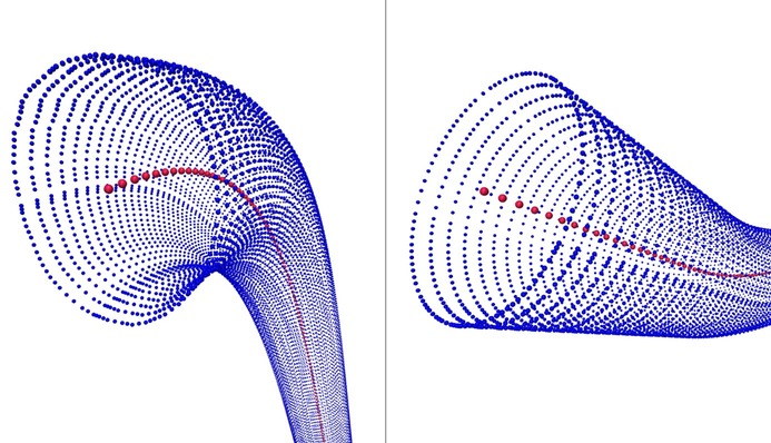
Figure 5. Two ends of the same connection. Generated “rings” of points transforming from a contour of a vessel section (left) into a circular shape (right)
Generating the actual connection 3D mesh
The result of the previous step was a collection of “rings” consisting of vertices. Knowing exactly the order of the “rings” as well as the consistent order of vertices in them, mesh cells can be created efficiently in a vectorized way using the “right-hand rule”.
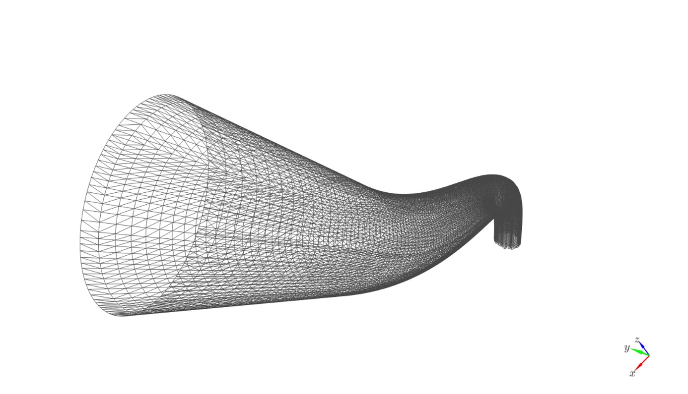
Figure 6. Generated connection mesh
Connecting the generated 3D mesh with the cut vessel mesh
There are multiple ways to connect the generated 3D mesh with the cut vessel mesh. The solution we chose was to treat corresponding boundary edges of a vessel and a generated connection as two closed polygons (“loops”) and then create a mesh that would bridge them. However, the real challenge was that meshes representing real anatomical structures could be unpredictable and appending artificially generated meshes to them may often result in non-manifold edges. Fixing non-manifold issues in meshes is a broad topic in itself and will not be covered in this article. Nor will be another significant problem which we also needed to handle which is merging multiple connection meshes starting from different branches and ending at the common target point.
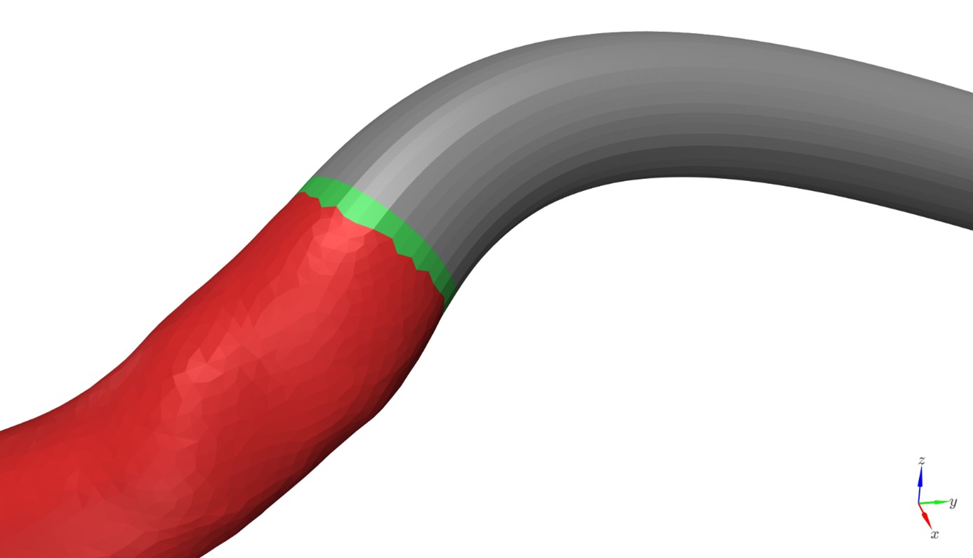
Figure 7. Cut model of a vessel (red), generated connection (gray) and the bridge between them (green)
3D mesh models of brain arteries – summary
The task of generating seamless connections from 3D mesh models of blood vessels was a truly interesting challenge. We were able to create the automated solution to difficult problems traditionally requiring sophisticated CAD tools and a qualified technician, by breaking the task down to smaller problems, using our broad expertise in Graylight Imaging as well as utilizing a suite of previously developed tools.
References:
[1] https://en.wikipedia.org/wiki/Frenet-Serret_formulas